Using Local Histograms to Alter Subject Tonal Range
Given the limited number of tonal values available in the RGB space, it is sometimes desirable to reallocate the available tonal range so that the subject area occupies relatively more and the background relatively less of the tonal range. Assuming the source image has the detail, this increases the tonal definition of the subject area at the expense of the background. Using local histograms enables the user to control the allocation precisely. Think of local histograms as the eyedropper tool for an area of the image.
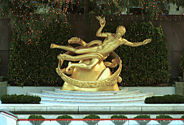
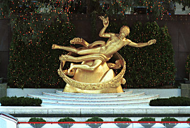
For example, in this image we want the statue to occupy more of the tonal space than the elements outside of it.
 |
 |
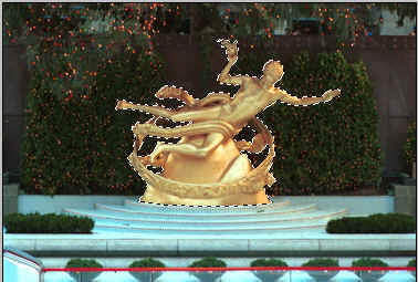
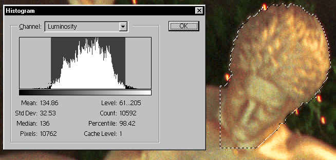
Step 1. First we select the statue so that we can define a histogram:
 |
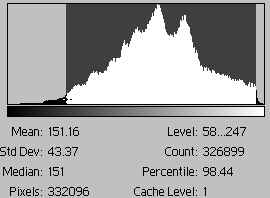 |
This image is an excellent candidate for this method because there is little overlap in tonal values between the subject and background, the statue histogram has a substantially different distribution than the background. Let's consider the interval 58 to 247, accounting for 98% of the subject's pixels (consider the other 2% noise pixels), as the tonal range of interest.
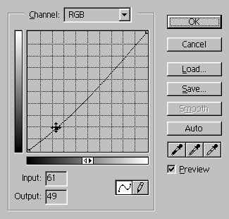
More specifically, the head occupies the range 61 to 205. The lower-ends of the local histograms are similar, but the upper-end of the statue as a whole is close to the extreme end. Clearly there is more tonal range available at the lower-end of the image a whole. Using the head's tonal range, we will expand the tonal range of the subject by reallocating 20% of the lower-end and 10% of the upper-end to the subject. Thus the tonal range of the head will be 49 to 210.
Step 2. Display the curves dialog box. Set an adjustment point such the input level is 61 and the output level is 49. This may be done either by using the mouse to drag the curve to the selected point or by entering the values directly into the edit fields.
Step 3. Set a second adjustment point such that the input level is 205 and the output level is 210.
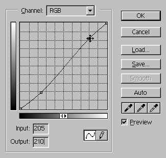
Step 4. You may save the curves file for re-use if you have another similar image.
 |
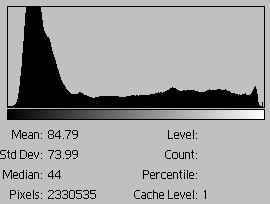 |
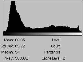
Because we gained contrast in the subject area at the expense of the shadow area, the base of hump representing the shadow area has narrowed as a result. Numerically, the mean and median have been decreased. The standard deviation, a proxy for the contrast of the image as a whole, has also increased. For comparison, the original scan and histogram are repeated. By employing local histograms, the subject is enhanced with respect to the background with no noticeable loss of image detail.
|
|
Here is a side-by-side comparison of detail from the original scan and curve adjusted scan:
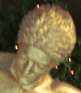
Without adjustment (w/o sharpening) |
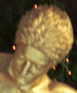
Adjusted (w/o sharpening) |
Of course, the above method isn't the only way to employ local histograms to allocate tonal range. A theoretically better alternative, when circumstances permit, is to use analog gain in increasing or decreasing contrast. For many applications, it's much faster and sufficient to run the eyedropper over the critical areas to obtain the necessary samples.
Notes
Since there is inevitably some overlap in pixel values between the subject and background areas, applying the curves will also affect some of the pixels outside of the subject area. This method is most effective when there is little tonal range overlap between the two areas.