|
Contents Understanding Image Histograms and Curves Histograms Histograms and Pixel Structure Using Histograms as a Scanner Tool Image Exposure and Tone Curves Changing Brightness and Contrast Interactive Demos Appendices The Photoshop Levels Function and Curves |
Now we'll return to the preview histograms we looked at earlier and apply our knowledge of image exposure and tone curves.
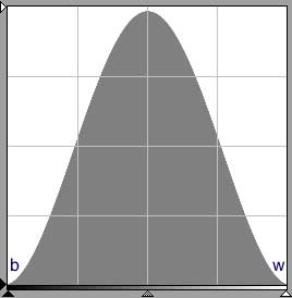 fig. 1
If you get a preview like this, just scan, no corrections are needed. The tonal range of the image (b to w) exactly matches the scanner's sensitivity (black to white triangle); the histogram's contour is smooth and continuous; there is no indication that tones have been clipped; and the mode is well away from the margins.
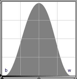 fig. 2
Fig. 2 is close enough. Just set the black and white points and scan.
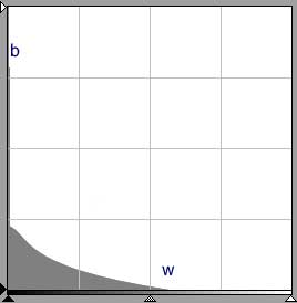 fig. 3a
 |
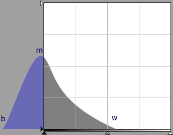 fig. 3b
|
For this image, some of the tones, as represented by the blue area in fig. 3b, are beyond the capabilities of the scanner. Scanned without adjustment, the blue area will appear as a long bar or cluster of bars adjacent to the vertical axis, as in fig. 3a. Fig. 3c is the tonal scale of the image prior to setting the white point (the black point is set already). Fig. 3d is the tonal scale after setting the white point through software.
|
fig. 3f |
Analog Gain Adjusting the analog gain merely means changing the luminance of the scanner's light source. Usually this means an increase so that sufficient light can pass through denser tones for the sensors to measure. You can conceptualize the effect of increasing analog gain on the image histogram as follows: Any pixel at point b is opaque black so increasing the luminance has no effect (no light passes through). Thus its value, or position on the graph, is unchanged. The lightest tone, w, is lightened the most so its value and thus its position is shifted right the most. If it is to be a true white, analog gain is adjusted until it meets the right margin, as in fig. 3e. Tones in between (m) are shifted right proportionately. |
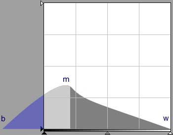 fig. 3e
To minimize this, we apply analog gain (i.e. increase the luminance of the LEDs) until the right edge of the histogram (w) touches the right margin, assuming that the tone represented by w is indeed white. This is also called setting the white point through hardware. Increasing analog gain has the effect of elongating the tonal scale (the distance from b to w) seen by the scanner. As a result more of the image's tones (light gray, fig. 3e) are shifted into the scanner's sensitivity range. Note that the tonal loss (blue area) has decreased and the tones properly imaged (gray areas) have increased. Without analog gain, a final scan with the distribution in fig. 3b will result in an image containing approximately 140 of the 256 available tones, whereas fig. 3e will contain all 256, as shown by fig. 3f. Compare tonal scale 3d with 3f. Figs. 3d and 3f are drawn with their widths proportionate to the number of tones in their images.
For an interactive simulation of the exposure adjustment process: Interactive Exposure Demo (requires Java enabled browser)
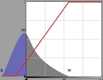 fig. 3g fig. 3g |
Adjusting analog gain implicitly applies a linear curve to the image in the analog domain. (Thus far, the curves we've discussed function in the digital domain.) In this example, setting analog gain to transform distribution 3b to 3e, we notionally apply the curve shown in 3g (red). An analog gain curve resembles that which is often used in setting the black-white points (characterized by the horizontal end segments), precisely our intent here. In this case, however, the effect of the curve extends to transform values outside the digital domain of the scanner (the super-imposed graph frame). (The inclusion of the graph frame is meant to help illustrate that scanning is a process of moving an image defined in the analog domain into the scanner's digital domain.) Note that the curve is notional and isn't displayable by the scanning program because this is a pre-scan adjustment.
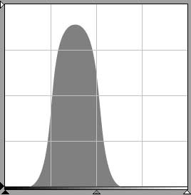 fig. 4
The problem with the histogram in fig. 4, often encountered with low-contrast films, is that it indicates a small range of tones. This is most often encountered in scanning color negative film. The approach to scanning low-contrast images is covered in A Brief Note on Scanning Color Negative Film
Temporary Curves
In addition to being used to form a final image, curves may also be used as a temporary expedient in evaluating an image. Returning to the earlier example, which was given to illustrate the limitations of using the monitor to evaluate the scan, suppose we want to make the differences visible:
 |
 |
In this case we can apply a curve with an 8:1 slope in the input interval 0 to 30 to both images to make the differences in the shadow areas more visible.
 |
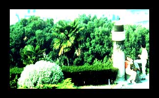 |
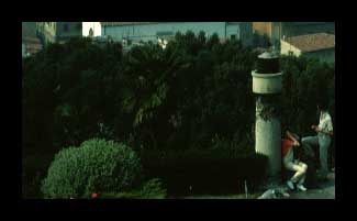
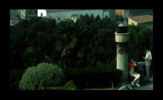
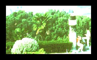
With a good scanner and careful control of exposure, images with full tonal ranges and shadow detail may be obtained, even from high contrast films, such as this one on Kodachrome 64:
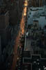 228 KB image
![]()
![]()