How to Interpret Area under the Curve

An important visual cue is the area under the curve. A histogram occupying a small area within its frame implies that a greater proportion of pixels have been imaged within a narrow band of tones. As a result, tonal separation may be diminished. This may be entirely consistent with the image, but if in addition it displays a bar of maximum height adjacent to the left or right margin, a problem is likely to have occurred.

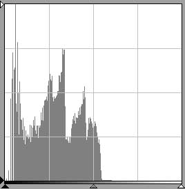
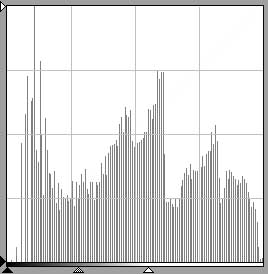
A typical continuous tone image will exhibit a relatively large area such as in the top histogram in fig. 12. In the bottom histogram in fig. 12, the relatively small area indicates a concentration in tones at or near the most frequent value. If two images are scanned at the same resolutions and have approximately the same crop area sizes, why are there differences in the absolute areas? After all, the histograms must account for an equal number of pixels and thus it seems they should have the same areas. As I mentioned earlier, the histogram is drawn within a frame of constant dimensions: there is a fixed vertical distance available to represent bar heights. The tonal value with the greatest frequency, the statistical mode, is set to this height no matter how many values are represented by this bar. The histogram's other bars are scaled relative to the mode. Thus a histogram with a small area indicates that the concentration at or near the mode has a much greater weight in representing the image's pixels. Another way to look at it would be to say that the vertical axes are scaled differently. If one were to label the two graphs, the bottom graph would have a greater number at its vertical maximum than the top graph. When the scaling difference is taken into account, the area under the curves would be the same.

This fortuitous combination of scaling about the mode and a fixed-frame histogram "normalizes" the histograms. In other words, this enables us to compare the tonal separations of two different images, independent of image size, by visually comparing the areas occupied by their histograms.

An average image will occupy a significant portion of the frame as in the histogram at left.

A concentration of tones, and thus a potential lack of tonal separation, is indicated by a histogram which occupies a relatively small area, left (white plus black). If the concentration, white for emphasis, occurs close to the left extreme, a problem with density range may be indicated. In this example, an area around the most frequent value (8 to 17) contains 37% of the image's pixels compared to 8% in the histogram above it.

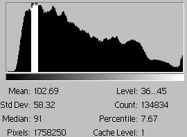
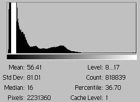
fig. 12

The evaluation of histogram areas is more useful in comparing successive scans of the same image.

fig. 13

fig. 13a

fig. 13b

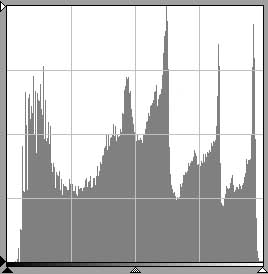
Figs. 13a and 13b are histograms for scans of the same hypothetical image, fig. 13. Fig. 13a shows that the scan of fig. 13 has resulted in an image with an exactly even dispersion of tones. The histogram occupies the entire frame. Fig. 13b, done with notionally incorrect settings or an inferior scanner, has a much smaller area because many of the scanned pixels have ended up in the bar adjacent to the left margin. Again, note that 13a and 13b account for the same number of pixels but have different areas because the vertical axes are scaled differently.

fig. 14a

fig. 14b

fig. 14c

Figs. 14 demonstrate the effects of two alternative methods of attaining a full range (black to white) of tones in an image. As previewed by the scanner, fig. 14a indicates an image with a narrow tonal range. By applying curves, fig. 14b is made from 14a by spreading the graph apart, much like an accordion, until it spans the full width of the graph. (Why this is done and how curves work is covered in the next section of this tutorial.) Gaps are left to fill the values vacated by the shifted bars. Note that since histogram 14b is 14a with its bars shifted -- gaps between its tones -- the area under the curve is the same. In contrast, fig. 14c achieves a full range of tones by adjusting the exposure through analog gain. It has a far greater area, about 80%, than fig. 14b and will have smoother tonal transitions. This is not to say that the image for 14b will be "bad," it depends on how much quality one needs to extract from the image.

The difference in areas in figs. 13 result from a concentration of tones. The difference in areas in figs. 14 result from gaps in data.

Everything else being equal for the same image, the scan with a histogram with greater area will contain more information and thus tend to exhibit superior tonal separation.

There's No Substitute for Practical Experience

I want to emphasize that there's no substitute for scanning on your own and analyzing your own scans and histograms. Start with images with various film types, lighting contrasts, and take notes. It's essential to be able to mentally associate the characteristics of an image with the resultant histogram, something that comes easily only with practice and experience.

What to Look for in The Histogram of A Well-Scanned Image of A Continuous Tone Picture

To summarize this section, this is what you look for in the histogram of a well-scanned continuous tone image:

	Absence of large gaps between values Usually caused by the application of curves. Minimized by additional bit-depth.
	Image makes use of available scanner density range Adjusted by analog gain.
	Smooth transitions from value to value Improved by bit-depth and multi-sampling (primarily in the shadow areas).

The final scan is performed when the scanner user cannot improve further on these criteria. The final scan serves as the basis of the production image(s), and therefore only coincidentally appears as ultimately intended. It is intended to obviate the need for rescans because it contains all of the readable data from the image.

Tone Curves or Setting Exposure -- An Interactive Demonstration